In
an earlier series of blog posts, I explored the question "What can we learn using RDF?". I
ended that series by concluding several things:
1. In order for the use of RDF to be beneficial, it needs to facilitate processing by semantic clients ("machines") that results in interesting inferences and information that would not otherwise be obvious to human users. We could call this the "
non-triviality" problem.
2. Retrieving information that isn't obvious is more likely to happen if the RDF is rich in object properties [1] that link to other IRI-identified resources and if those linked IRIs are from Internet domains controlled by different providers. We could call this the "
Linked Data" problem: we need to break down the silos that separate the datasets of different providers. We could reframe by saying that the problem to be solved is the lack of persistent, unique identifiers, lack of consensus object properties, and lack of the will for people to use and reuse those identifiers and properties.
3. RDF-enabled machine reasoning will be beneficial if the entailed triples allow the construction of more clever or meaningful queries, or if they state relationships that would not be obvious to humans. We could call this the "
Semantic Web" problem.
RDF has now been around for about fifteen years, yet it has failed to gain the kind of traction that the HTML-facilitated, human-oriented Web attained in its first fifteen years. I don't think the problem is primarily technological. The necessary standards (RDF, SPARQL, OWL) and network resources are in place, and computing and storage capabilities are better than ever. The real problem seems to be a social one. In the community within which I function (biodiversity informatics), with respect to the Linked Data problem, we have failed to adequately scope what the requirements are for a "good" object properties, and failed to settle on a usable system for facilitating discovery and reuse of identifiers. With respect to the Semantic Web problem, there has been relatively little progress on discussing as a community [2] the nature of the use cases we care about, and how the adoption of particular semantic technologies would satisfy them. What's more, with the development of
schema.org and
JSON-LD, there are those who question whether the Semantic Web problem is even relevant.
This blog post ties together the old "What can we learn using RDF?" theme with theme of
this new blog series ("Shiny new toys") by examining a design choice about object properties that Cam Webb and I made when we created
Darwin-SW. I show how we can play with the "shiny new toys" (Darwin-SW 0.4, the Bioimages RDF dataset, and the Heard Library Public SPARQL endpoint) to investigate the practicality of that choice. I end by pondering how that design choice is related to the RDF problems I listed above.
Why is it called "Darwin-SW"?
In my previous blog post, I mentioned that instances of
Darwin Core classes in
Bioimages RDF are linked using
a graph model based mostly on the
Darwin-SW ontology (DSW). A primary function of Darwin-SW is to provide the object properties that are missing from Darwin Core. For example, Darwin Core itself does not provide any way to link an Organism with its Identifications or its Occurrences.
If linking were the only purpose of Darwin-SW, then why isn't it called "Darwin-LD" (for "Darwin Linked Data") instead of Darwin-SW (for "Darwin Semantic Web")? When Cam Webb and I developed it, we wanted to find out what kinds of properties we could assign to the DSW terms that would satisfy some use cases that were interesting to us. We were interested in at leveraging at least some of the capabilities of the Semantic Web in addition to facilitating Linked Data.
Compared to
OBO Foundry ontologies, DSW is a fairly light-weight ontology. It doesn't generate a lot of entailments because it uses
OWL properties somewhat sparingly, but there are specific term properties that generate important entailments that help us satisfy our use cases. [4] Darwin-SW declares some classes to be disjoint, establishes the key transitive properties
dsw:derivedFrom and
dsw:hasDerivative, declares ranges and domains for many properties, and
defines pairs of object properties that are declared to be inverses. It is the last item that I'm going to talk about specifically in this blog post. (I may talk about the others in later posts.)
What are inverse properties?
Sometimes a vocabulary defines a single object property to link instances of classes of subject and object resources. For example,
Dublin Core defines the term
dcterms:publisher to link a resource to the Agent that published it:
On the other hand, Dublin Core also defines the terms
dcterms:hasPart and
dcterms:isPartOf, which can be used to link a resource to some other resource that is included within it.
In the first case of
dcterms:publisher, there is only one way to write a triple that links the two resources, e.g.
<http://bioimages.vanderbilt.edu/hessd/e5397>
dcterms:publisher <http://biocol.org/urn:lsid:biocol.org:col:35115>.
But in the second case, there are two ways to create the linkage, e.g.
<http://rs.tdwg.org/dwc/terms/>
dcterms:hasPart <http://rs.tdwg.org/dwc/terms/lifeStage>.
or
<http://rs.tdwg.org/dwc/terms/lifeStage>
dcterms:isPartOf <http://rs.tdwg.org/dwc/terms/>.
Because the terms
dcterms:hasPart and
dcterms:isPartOf link the two resources in opposite directions, they could be considered inverse properties. You have the choice of using either one to perform the linking function.
If a vocabulary creator like
DCMI provides two apparent inverse properties that can be used to link a pair of resources in either direction, that brings up an important question. If a user asserts that
<http://rs.tdwg.org/dwc/terms/>
dcterms:hasPart <http://rs.tdwg.org/dwc/terms/lifeStage>.
is it safe to assume that
<http://rs.tdwg.org/dwc/terms/lifeStage>
dcterms:isPartOf <http://rs.tdwg.org/dwc/terms/>.
is also true? It would make sense to think so, but DCMI actually never explicitly states that asserting the first relationship entails that the second relationship is also true. Compare that to the situation in the FOAF vocabulary, which defines the terms
foaf:depicts and
foaf:depiction
In contrast to the Dublin Core
dcterms:hasPart and
dcterms:isPartOf properties, FOAF explicitly declares
foaf:depicts owl:inverseOf foaf:depiction.
in the
RDF definition of the vocabulary. So stating the triple
http://bioimages.vanderbilt.edu/vanderbilt/7-314
foaf:depiction http://bioimages.vanderbilt.edu/baskauf/79653.
entails
http://bioimages.vanderbilt.edu/baskauf/79653
foaf:depicts http://bioimages.vanderbilt.edu/vanderbilt/7-314.
regardless of whether the second triple is explicitly stated or not.
Why does this matter?
When the creator of a vocabulary offers only one property that
can be used to link a certain kind of resource to another kind of
resource, data consumers can know that they will always find all of the linkages between the two kinds of resources when they search for them. The query
SELECT ?book WHERE {
?book dcterms:publisher ?agent.
}
will retrieve every case in a dataset where a book has been linked to its publisher.
However, when the creator of a vocabulary offers two choices of properties that can be used to link a certain kind of resource to another kind of resource, there is no way for a data consumer to know whether a particular dataset producer has expressed the relationship in one way or the other. If a dataset producer asserts only that
<http://rs.tdwg.org/dwc/terms/>
dcterms:hasPart <http://rs.tdwg.org/dwc/terms/lifeStage>.
but a data consumer performs the query
SELECT ?term WHERE {
?term dcterms:isPartOf ?vocabulary.
}
the link between vocabulary and term asserted by the producer will not be discovered by the consumer. In the absence of a pre-established agreement between the producer and consumer about which property term will always be used to make the link, the producer must express the relationship both ways, e.g.
# producer's data
<http://rs.tdwg.org/dwc/terms/>
dcterms:hasPart <http://rs.tdwg.org/dwc/terms/lifeStage>.
<http://rs.tdwg.org/dwc/terms/lifeStage>
dcterms:isPartOf <http://rs.tdwg.org/dwc/terms/>.
if the producer wants to ensure that consumers will always discover the relationship. In order for consumers to ensure that they find every case where terms are related to vocabularies, they must perform a more complicated query like:
SELECT ?term WHERE {
{?term dcterms:isPartOf ?vocabulary.}
UNION
{?vocabulary dcterms:hasPart ?term.}
}
This is really annoying. If a lot of inverse properties are involved, either the producer must assert a lot of unnecessary triples or the consumer must write really complicated queries. For the pair of Dublin Core terms, this is the only alternative in the absence of a convention on which of the two object properties should be used.
However, for the pair of FOAF terms, there is another alternative. Because the relationship
foaf:depicts owl:inverseOf foaf:depiction.
was asserted in the FOAF vocabulary definition, a data producer can safely assert the relationship in only one way IF the producer is confident that the consumer will be aware of the
owl:inverseOf assertion AND if the consumer performs reasoning on the producer's graph (i.e. a collection of RDF triples). By "performs reasoning", I mean that the consumer uses some kind of semantic client to materialize the missing, entailed triples and add them to the producer's graph. If the producer asserts
http://bioimages.vanderbilt.edu/baskauf/79653
foaf:depicts http://bioimages.vanderbilt.edu/vanderbilt/7-314.
and the consumer conducts the query
SELECT ?plant WHERE {
?plant foaf:depiction ?image.
}
the consumer will discover the relationship if pre-query reasoning materialized the entailed triple
http://bioimages.vanderbilt.edu/vanderbilt/7-314
foaf:depiction http://bioimages.vanderbilt.edu/baskauf/79653.
and included it in the dataset that was being searched.
Why did Darwin-SW include so many inverse property pairs?
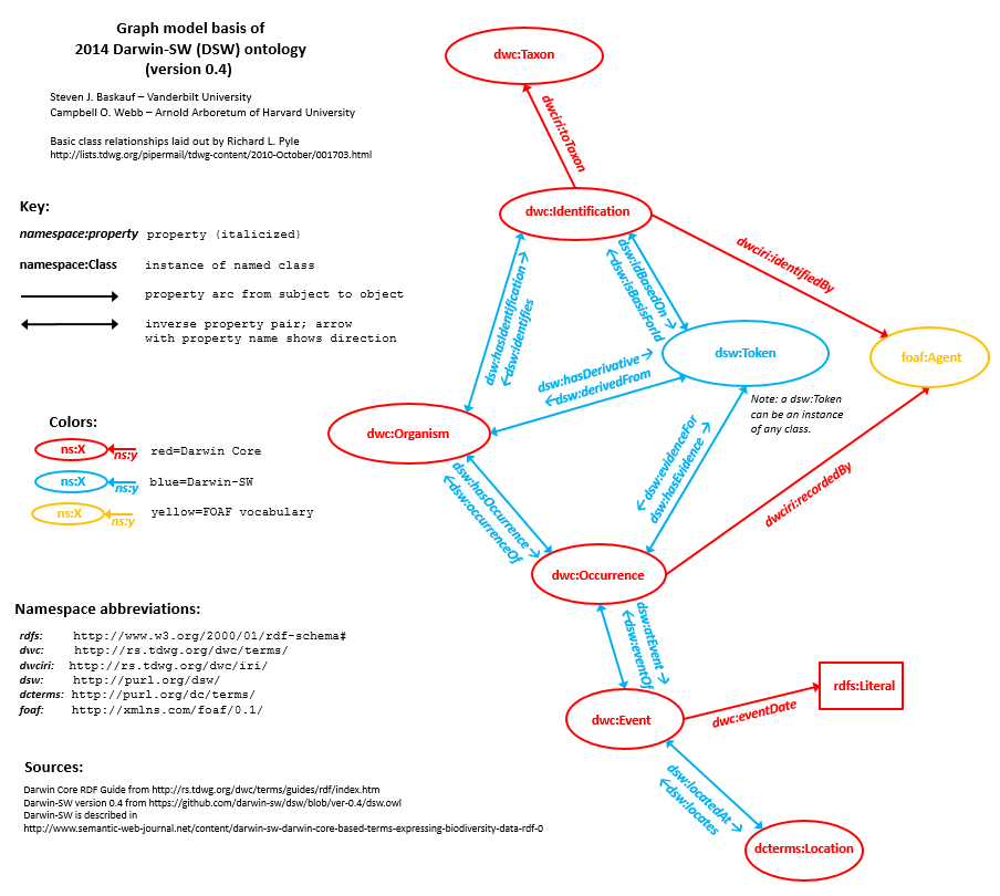
Examination of the graph model above shows that DSW is riddled with pairs of inverse properties. Like
foaf:depicts and
foaf:depiction, each property in a pair is declared to be
owl:inverseOf its partner. Why did we do that when we created Darwin-SW?
Partly we did it as a matter of convenience. If you are describing an organism, it is slightly more convenient to say
http://bioimages.vanderbilt.edu/vanderbilt/7-314
a dwc:Organism;
dwc:organismName "Bicentennial Oak"@en;
dsw:hasDerivative http://bioimages.vanderbilt.edu/baskauf/79653.
than to have to say
http://bioimages.vanderbilt.edu/vanderbilt/7-314
a dwc:Organism;
dwc:organismName "Bicentennial Oak"@en.
http://bioimages.vanderbilt.edu/baskauf/79653
dsw:derivedFrom http://bioimages.vanderbilt.edu/vanderbilt/7-314.
The other reason for making it possible to establish links in either direction is somewhat philosophical. Why did DCMI create a property that links documents and their publishers in the direction where the document was the subject and not the other way around? Probably because Dublin Core is all about describing the properties of documents, and not so much about describing agents (that's FOAF's thing). Why did
TDWG create the Darwin Core property
dwciri:recordedBy that links Occurrences to the Agents that record them in the direction where Occurrence is the subject and not the other way around? Because TDWG is more interested in describing Occurrences than it is in describing agents. In general, vocabularies define object properties in a particular direction so that the kind of resource their creators care about the most is in the subject position of the triple. TDWG has traditionally been specimen- and Occurrence-centric, whereas Cam and I have the attitude that in a graph-based RDF world, there isn't any center of the universe. It should be possible for any resource in a graph to be considered the subject of a triple linking that resource to another node in the graph. So we created DSW so that users can always chose an object property that places their favorite Darwin Core class in the subject position of the triple.
Is creating a bunch of inverse property pairs a stupid idea?
In creating DSW, Cam and I didn't claim to have a corner on the market of wisdom. What we wanted to accomplish was to lay out a possible, testable solution for the problem of linking biodiversity resources, and then see if it worked. If one assumes that it isn't reasonable to expect data producers to express relationships in both directions, nor to expect consumers to always write complex queries, the feasibility of minting inverse property pairs really depends on whether one "believes in" the Semantic Web. If one believes that carrying out machine reasoning is feasible on the scale in which the biodiversity informatics community operates, and if one believes that data consumers (or aggregators who provide those data to consumers) will routinely carry out reasoning on graphs provided by producers, then it is reasonable to provide pairs of properties having
owl:inverseOf relationships. On the other hand, if data consumers (or aggregators who provide data to consumers) can't or won't routinely carry out the necessary reasoning, then it would be better to just deprecate one of the properties of each pair so that there will never be uncertainty about which one data producers will use.
So part of the answer to this question involves discovering how feasible it is to conduct reasoning of the sort that is required on a graph that is of a size that might be typical for biodiversity data producers.
Introducing the reasoner
"Machine reasoning" can mean several things. On type of reasoning is to determine unstated triples that are entailed by a graph (see
this blog post for thoughts on that). Another type of reasoning is to determine whether a graph is consistent (see
this blog post for thoughts on that). Reasoning of the first sort is carried out on graphs by software that has been programmed to apply entailment rules. It would be tempting to think that it would be good to have a reasoner that would determine all possible entailments. However, that is undesirable for two reasons. The first is that applying some entailment rules may have undesired consequences (see
this blog post for examples; see
Hogan et al. 2009 for examples of categories of entailments that they excluded). The second is that it may take too long to compute all of the entailments. For example, some uses of
OWL Full may be undecidable (i.e. all entailments are not computable in a finite amount of time). So in actuality, we have to decide what sort of entailment rules are important to us, and find or write software that will apply those rules to our graph.
A number of reasoners have been developed to efficiently compute entailments and determine consistency. One example is
Apache Jena. There are various strategies that have been employed to optimize the process of reasoning. If a query is made on a graph, a reasoner can compute entailments "on the fly" as it encounters triples that entail them. However, this process would slow down the execution of every query. Alternatively, a reasoner could compute the set of entailed triples using the entire data graph and save those "materialized" triples in a separate graph. This might take more time than computing the entailments at query time, but it would only need to be done once. After the entailed triples are stored, queries could be run on the union of the data graph and the graph containing the materialized entailed triples with little effect on the time of execution of the query.
This strategy is called "forward chaining".
Creating a reasoner using a SPARQL endpoint
One of the "shiny new toys" I've been playing with is the public
Vanderbilt Heard Library SPARQL endpoint that we set up as part of a
Dean's Fellow project. The endpoint is set up on a Dell PowerEdge 2950 with 32GB RAM and uses Callimachus 1.4.2 with an Apache frontend. In the previous blog post, I talked about the
user-friendly web page that we made to demonstrate how SPARQL could be used to query the Bioimages RDF (another of my "shiny new toys"). In the
Javascript that makes the web page work, we used the SPARQL SELECT query form to find resources referenced in triples that matched a graph pattern (i.e. set of triple patterns). The main query that we used screened resources by requiring them to be linked to other resources that had particular property values. This is essentially a Linked Data application, since it solves a problem by making use of links between resources (although it would be a much more interesting one if links extended beyond the Bioimages RDF dataset).
The SPARQL CONSTRUCT query form asks the endpoint to return a graph containing triples constrained by the graph pattern specified in the WHERE clause of the query. Unfortunately, CONSTRUCT queries can't be carried out by pasting them into the
blank query box of the Heard Library endpoint web page. The endpoint
will carry out CONSTRUCT queries if they are submitted using
cURL or some other application that allows you to send HTTP GET requests directly. I used the
Advanced Rest Client Chrome extension, which displays the request and response headers and also measures the response time of the server. If you are trying out the examples I've listed here and don't want to bother figuring out how to configure an application send and receive the data related to CONSTRUCT queries, you can generally replace
CONSTRUCT {?subject ex:property ?object.}
with
SELECT ?subject ?object
and paste the modified query in the blank query box of the endpoing web page. The subjects and objects of the triples that would have been constructed will then be shown on the screen. It probably would also be advisable to add
LIMIT 50
at the end of the query in case it generates thousands of results.
In the previous section, I described a
forward chaining reasoner as performing the following functions:
1. Apply some entailment rules to a data graph to generate entailed triples.
2. Store the entailed triples in a new graph.
3. Conduct subsequent queries on the union of the data graph and the entailed triple graph.
These functions can be duplicated by a SPARQL endpoint responding to an appropriate CONSTRUCT query if the WHERE clause specifies the entailment rules. The endpoint returns the graph of entailed triples in response to the query, and that graph can be loaded into the triple store to be included in subsequent queries.
Here is the start of a query that would materialize triples that are entailed by using properties that are declared to have an
owl:inverse relationship to another property:
CONSTRUCT {?Resource1 ?Property2 ?Resource2.}
WHERE {
?Property1 owl:inverseOf ?Property2.
?Resource2 ?Property1 ?Resource1.
}
To use this query, the RDF that defines the properties (e.g. the FOAF vocabulary RDF document) must be included in the triplestore with the data. The first triple pattern binds instances of declared inverse properties (found in the vocabulary definitions RDF) to the variables ?Property1 and ?Property2. The second triple pattern binds subjects and objects of triples containing ?Property1 as their predicate to the variables ?Resource2 and ?Resource1 respectively. The endpoint then constructs new triples where the subject and object positions are reversed and inserts the inverse property as the predicate.
There are two problems with the query as it stands. The first problem is that the query generates ALL possible triples that are entailed by triples in the dataset that contain ?Property1. Actually, we only want to materialize triples if they don't already exist in the dataset. In SPARQL 1.0, fixing this problem was complicated. However, in SPARQL 1.1, it's easy. The MINUS operator removes matches if they exist in some other graph. Here's the modified query:
CONSTRUCT {?Resource1 ?Property2 ?Resource2.}
WHERE {
?Property1 owl:inverseOf ?Property2.
?Resource2 ?Property1 ?Resource1.
MINUS {?Resource1 ?Property2 ?Resource2.}
}
The first two lines binds resources to the same variables as above, but the MINUS operator eliminates bindings to the variables in cases where the triple to be constructed already exists in the data. [5]
The other problem is that
owl:inverseOf is symmetric. In other words, declaring:
<property1> owl:inverseOf <property2>.
entails that
<property2> owl:inverseOf <property1>.
In a vocabulary definition, it should not be necessary to make declarations in both directions, so vocabularies generally only declare one of them. Since the SPARQL-based reasoner we are creating is ignorant of the semantics of
owl:inverseOf, we need to take additional steps to make sure that we catch entailments based on properties that are either the subject
or the object of an
owl:inverseOf declaration. There are several ways to do that.
One possibility would be to simply materialize all of the unstated triples that are entailed by the symmetry of
owl:inverseOf. That could be easily done with this query:
CONSTRUCT {?Property1 owl:inverseOf ?Property2.}
WHERE {
?Property2 owl:inverseOf ?Property1.
MINUS {?Property1 owl:inverseOf ?Property2.}
}
followed by running the modified query we created above.
An alternative to materializing the triples entailed by the symmetry of
owl:inverseOf would be to run a second query:
CONSTRUCT {?Resource1 ?Property2 ?Resource2.}
WHERE {
?Property2 owl:inverseOf ?Property1.
?Resource2 ?Property1 ?Resource1.
MINUS {?Resource1 ?Property2 ?Resource2.}
}
similar to the earlier one we created, but with the subject and object positions of
?Property1 and
?Property2 are reversed. It might be even better to combine both forms into a single query:
CONSTRUCT {?Resource1 ?Property2 ?Resource2.}
WHERE {
{?Property1 owl:inverseOf ?Property2.}
UNION
{?Property2 owl:inverseOf ?Property1.}
?Resource2 ?Property1 ?Resource1.
MINUS {?Resource1 ?Property2 ?Resource2.}
}
Hooray! We have created a simple reasoner to materialize entailed by
owl:inverseOf properties! Flushed with excitement, I rush to send the query to the Heard Library SPARQL endpoint to try it on the Bioimages RDF ...
... only to sit there waiting until the server times out.
What happened? Although this kind of query works on small "practice" datasets, there are too many triples in the Bioimages dataset for the endpoint to complete the task in the time allowed in the system settings (which I think is limited to 60 seconds).
A more modest SPARQL reasoner
After this initial failure, perhaps we should scale back our expectations and figure out what was making the query take too long.
First, it would be good to have a way to determine the scope of what we were asking the endpoint to do. SPARQL provides a way to find out how many times an expression has bound: the COUNT function. It would also be good to make sure that the query is being done only on the triples we care about (the Bioimages data). Here is a query that will determine the number of triples contained in the graph that is bundled in the
bioimages-rdf.zip file on the
Bioimages GitHub repository (release 2014-07-22,
http://dx.doi.org/10.5281/zenodo.21009):
PREFIX foaf: <http://xmlns.com/foaf/0.1/>
PREFIX ac: <http://rs.tdwg.org/ac/terms/>
PREFIX dwc: <http://rs.tdwg.org/dwc/terms/>
PREFIX dwciri: <http://rs.tdwg.org/dwc/iri/>
PREFIX dsw: <http://purl.org/dsw/>
PREFIX Iptc4xmpExt: <http://iptc.org/std/Iptc4xmpExt/2008-02-29/>
PREFIX rdfs: <http://www.w3.org/2000/01/rdf-schema#>
PREFIX dc: <http://purl.org/dc/elements/1.1/>
PREFIX dcterms: <http://purl.org/dc/terms/>
PREFIX dcmitype: <http://purl.org/dc/dcmitype/>
SELECT (COUNT(?subject) AS ?count)
FROM <http://rdf.library.vanderbilt.edu/bioimages/images.rdf>
FROM <http://rdf.library.vanderbilt.edu/bioimages/organisms.rdf>
FROM <http://rdf.library.vanderbilt.edu/bioimages/baskauf.rdf>
FROM <http://rdf.library.vanderbilt.edu/bioimages/thomas.rdf>
FROM <http://rdf.library.vanderbilt.edu/bioimages/uri.rdf>
FROM <http://rdf.library.vanderbilt.edu/bioimages/kirchoff.rdf>
FROM <http://rdf.library.vanderbilt.edu/bioimages/ncu-all.rdf>
FROM <http://rdf.library.vanderbilt.edu/bioimages/dsw.owl>
FROM <http://rdf.library.vanderbilt.edu/bioimages/dwcterms.rdf>
FROM <http://rdf.library.vanderbilt.edu/bioimages/local.rdf>
FROM <http://rdf.library.vanderbilt.edu/bioimages/stdview.rdf>
WHERE {
?subject ?predicate ?object.
}
A few notes about this query:
1. The PREFIX declarations include more namespaces than are necessary for any particular query included in this blog post. I've included all of the ones that I typically use when querying the Bioimages RDF dataset so that it would be easier for you to make up your own queries. Typically, a PREFIX declaration must be included in any SPARQL query in which that namespace is abbrevated. However, the
Callimachus Web interface for the Heard Library endpoint (the blank box page) will "remember" prefixes once they have been declared in a query, so if you are using the Web interface, you only need to declare them once (per session?). To be safe, you can just paste this set of PREFIX declarations above into any of the queries I list below.
2. The FROM clause includes a particular graph in the dataset to be queried. Although I won't show these FROM clauses in the example queries that follow, you should place that set of FROM clauses between the SELECT or DESCRIBE clause and the WHERE clause in the example queries. The queries may work without doing this, but without the FROM claueses, the queries might pick up random triples that Callimachus has left lying around in the triplestore.
3. The expression
(COUNT(?subject) AS ?count) calculates the number of expressions bound to the
?subject variable and then binds that integer value to the
?count variable.
Running this query against the Bioimages dataset produces an integer value of 1488578 and takes 9793 ms to execute.[6] So performing a query that binds about 1.5 million triples takes Callimachus about 10 seconds. The time to execute seems to depends primarily on the number of sets of bound variables as can be seen if you rerun the query without the
FROM <http://rdf.library.vanderbilt.edu/bioimages/images.rdf>
clause. This time it only takes 1721 ms because the
images.rdf file contains the lion's share of the triples in the dataset (1211642, to be exact).
Just for fun, you can play with the COUNT function by running a more complicated query designed to list all of the photographers whose work has been contributed to Bioimages, ordered by the number of images contributed:
SELECT ?photographerName (COUNT(?image) AS ?count)
WHERE {
?image a dcmitype:StillImage.
?image dc:creator ?photographerName.
}
GROUP BY ?photographerName
ORDER BY DESC(?count)
This query also illustrates the use of two more useful SPARQL clauses: GROUP BY and ORDER BY.
Now back to business. To limit this investigation to a smaller number of triples, I'm going to investigate a set of inverse properties that involves only Organisms and not images. This query
SELECT (COUNT(?subject) AS ?count)
WHERE {
?subject a dwc:Organism.
}
tells us how many Organisms are described in the Bioimages dataset (3316) and changing "
a dwc:Organism" to "
a dcmitype:StillImage" tells us how many images are described (13597). There are an average of about 4 images per Organism, with Organisms and images having approximately equal numbers of properties. So limiting the investigation to Organism properties and eliminating image properties reduces the scope of the query considerably.
I'm going to investigate this part of the
Bioimages RDF graph model (which comes from
the DSW graph model):
Organism Occurrences are documented by three different classes of things in the Bioimages dataset. You can discover them using this query.
SELECT DISTINCT ?class
WHERE {
?occurrence a dwc:Occurrence.
?occurrence dsw:hasEvidence ?thing.
?thing a ?class.
}
In RDF/Turtle (on which SPARQL triple patterns are based), "
a" is syntatic sugar for "
rdf:type", so this query tells us what types (classes) of things provide evidence for Occurrences of Organisms (called "Tokens" in DSW). There are three distinct types of things: Organisms that are living specimens (mostly trees in the Vanderbilt arboretum), still images (most of the records), and preserved specimens (a few records of trees documented by specimens in the University of North Carolina [NCU)] Herbarium).
In an earlier version of the Bioimages RDF data, I was careful to always link Organisms and Occurrences with both of the relevant inverse properties:
dsw:hasOccurrence and
dsw:occurrenceOf. However, in the current version I decided to use only the one property that was the most convenient for the way I generated the RDF:
dsw:hasOccurrence.
dsw:occurrenceOf is grayed out in the Bioimages RDF graph model diagram because although triples involving it are entailed, they are not usually materialized in the dataset. [7] The exception to this are the Occurrences documented by the NCU preserved specimens - the file containing the triples describing them (
ncu-all.rdf) was basically hand-constructed as a test and includes
dsw:occurrenceOf properties.
We can find out how many times
dsw:hasOccurrence was used in the dataset with this query:
SELECT (COUNT(?occurrence) AS ?count)
WHERE {
?organism dsw:hasOccurrence ?occurrence.
}
There are 4096 instances. As expected, substituting
dsw:occurrenceOf for
dsw:hasOccurrence finds the 27 instances used in the descriptions of the Occurrences documented by the 27 NCU specimens. To test the method of constructing entailed triples using SPARQL CONSTRUCT, we can use the query:
CONSTRUCT {?organism dsw:hasOccurrence ?occurrence.}
WHERE {
?occurrence dsw:occurrenceOf ?organism.
}
This query should construct the triples entailed by the 27 triples in the NCU specimen subgraph having dsw:occurrenceOf as their predicate, and it does - in only 603 ms. The time is short whether the images.rdf triples are added to the queried dataset using
FROM <http://rdf.library.vanderbilt.edu/bioimages/images.rdf>
or not. Even though including the images.rdf triples increases the size of the queried dataset by a factor of about 5, it does not increase the number of triples bound by the triple pattern
?occurrence dsw:occurrenceOf ?organism.
so there is little effect on the speed of execution. In order to make this query do what we actually want, we need to remove triples that are already included in the dataset:
CONSTRUCT {?organism dsw:hasOccurrence ?occurrence.}
WHERE {
?occurrence dsw:occurrenceOf ?organism.
MINUS {?organism dsw:hasOccurrence ?occurrence.}
}
Since every link between Organisms and Occurrences should already be documented by a triple containing
dsw:hasOccurrence, this query should produce no results. Surprisingly, it
does produce a single result in 732 ms:
<rdf:Description rdf:about="http://bioimages.vanderbilt.edu/ind-kirchoff/mason03">
<dsw:hasOccurrence rdf:resource="http://bioimages.vanderbilt.edu/specimen/ncu592813#occ" />
</rdf:Description>
Upon further investigation, I found that this unexpected triple was caused by my mistyping of "ncu592831" instead of "ncu592813". So the query correctly materialized the one entailed triple that wasn't already included in the dataset.
Now let's try the more useful query that should materialize the many missing entailed triples that contain
dsw:occurrenceOf:
CONSTRUCT {?occurrence dsw:occurrenceOf ?organism.}
WHERE {
?organism dsw:hasOccurrence ?occurrence.
MINUS {?occurrence dsw:occurrenceOf ?organism.}
}
It takes a lot longer for the server to run this query (5477 ms) because it has to construct a lot more triples than in the previous query. The query does correctly remove the pre-existing 26 "dsw:occurrenceOf" triples from the set of 4096 triples that are entailed by triples containing dsw:hasOccurrence as their predicate. Again, it makes little difference in the execution time whether the many images.rdf triples are included in the whole dataset or not, since none of them are bound in the query.
OK, the endpoint was able to handle reasoning on this scale within the timeout limits. Let's try something more demanding.
Playing harder with the toys
Earlier, we used the
dsw:hasEvidence linking predicate to find out what kinds of things were used to document occurrences. There are more
dsw:hasEvidence links than there are
dsw:hasOccurrence links because there are more documentary images in the dataset than there are Occurrences. We can find out how many
dsw:hasEvidence links there are by this query:
SELECT (COUNT(?token) AS ?count)
WHERE {
?occurrence dsw:hasEvidence ?token.
}
In 351 ms we find out that there are 13827. We can check on the number of links that were made in the opposite direction by:
SELECT (COUNT(?token) AS ?count)
WHERE {
?token dsw:evidenceFor ?occurrence.
}
and in 350 ms we get the answer: 13624. The difference between these two results tells us that there are at least 203 unmaterialized, entailed triples having
dsw:evidenceFor as their predicate. Here's the reason: although in case of images the links between Occurrences and the Tokens that serve as evidence for them them are made in both directions, in the case of living specimens in arboreta I didn't explicitly make the link in the direction that used
dsw:evidenceFor. There is no particularly good reason for that choice - as a data producer I was just using the prerogative that Darwin-SW gave me. So this would be an excellent opportunity to fix that problem using forward-chaining reasoning. I should be able to construct the missing 203 "
dsw:evidenceFor" triples with this query:
CONSTRUCT {?occurrence dsw:hasEvidence ?token.}
WHERE {
?token dsw:evidenceFor ?occurrence.
MINUS {?occurrence dsw:hasEvidence ?token.}
}
Alas, we have pushed our "shiny new toy" (the Heard Library SPARQL endpoint) too far. After 60442 ms, the endpoint times out and we get nothing. There were just too many bindings for the endpoint to complete the processing in the allowed time.
Some thoughts about time needed to reason...
Using my homemade SPARQL reasoner to materialize missing triples entailed by use of inverse properties worked fine when the number of links documented by the inverse properties was not too big. It was able to generate about 4000 entailed triples while checking them against about another 4000 existing triples that expressed the link using the inverse property, and it did so in about 5.5 seconds. However, when that number was increased by about a factor of 3.5 (to about 14000 triples), the endpoint timed out after 60 seconds. Clearly the relationship between the number of triples involved and the time it takes to execute is not linear. This makes sense if one considers what the MINUS operator does. The MINUS operator compares the set of variable bindings that satisfy one graph pattern with the set that satisfies a second graph pattern. It then removes the second set of bindings from the first. If each binding from the first graph has to be checked against each binding from the second, and the time it takes to make each comparison is the same, the time to make the comparison should be proportional to the square of the number of bindings (assuming that the number of bindings in the first graph are similar to the second). Based on this seat-of-the-pants guesstimate, increasing the number of triples from 4000 to 14000 would increase the time required from about 5.5 seconds to 5.5*3.5^2 seconds or 67 seconds, which would push it just beyond the 60 second timeout of the endpoint. I haven't attempted to test this by having the timeout setting lengthened.
The point is that the time required to carry out reasoning on a graph that contains 1.5 million triples is not negligible. Reasoner performance could be improved by using a better computer or a more efficient algorithm than one based on Callimachus SPARQL queries; that is, use software actually designed to conduct reasoning of this sort. But even with these kinds of improvements, reasoning on a dataset with a more realistic size could take a long time. I spent some time Googling to find some examples where "real" reasoners were used on "real" datasets to try to get a feel for the time that would be required to reason over large assertional datasets (i.e. instance data) as opposed to large terminological datasets (complex ontologies like the OBO biomedical ontologies). After wasting a lot of time, I ended up falling back on the Hogan et al. (2009) paper [8], which I've brought up in previous blog posts. In their study, they collected about a billion (i.e. 10^9) triples from "the wild" by scraping the Web. This is about 3 orders of magnitude larger than the Bioimages dataset. They applied a restricted set of entailment rules (see their section 3.3 and following sections) to the data (see their section 3.5) and let their algorithm rip. When reasoning was done on the billion triples using a single computer (see their section 3.6), they materialized about a billion new entailed triples in 19.5 hours. Using 1 master and 8 slave computers, they were able to compute the same entailed triples in 3.5 hours.
The Hogan et al. triples were fairly "dirty" since they were harvested from all over the web and the reasoning process they applied was much more complex than reasoning only the triples entailed by inverse property declarations. So simpler reasoning on cleaner data might take less time. Nevertheless, it clearly takes a while when reasoning has to be applied to many triples. I tried to imagine the size of the dataset that would result if all of the
Occurrence records in GBIF were described using RDF. As of today (2015-07-26), GBIF has 566 589 120 Occurrence records. It takes about 100 triples to describe each instance of a resource (image or Organism) in the Bioimages RDF dataset. At that rate, it would require about 50 000 000 000 (5*10^10 or 50 billion) triples to express the GBIF Occurrence dataset as RDF. That's about 50 times larger than the Hogan et al. dataset. If the processing time were linearly related to number of triples and the nature of the reasoning were similar to that performed by Hogan et al., it could take about 1000 hours (about 6 weeks) for the Hogan et al. seven-computer master/slave reasoner configuration to reason over the GBIF dataset. If the time required were worse than linear (as it appears with my homemade SPARQL reasoner), then the time could be much longer. If the reasoning process were much simpler because fewer entailment rules were used, then the time could be a lot shorter.
Another major consideration is whether the reasoning needs to be applied repeatedly to the entire dataset, or only once to new data when it is added to the dataset. When
forward chaining is used by a reasoner, the entailed materialized triples only have to be computed once for a fixed dataset. However, if triples are added to the original dataset, the entailed triples may need to be recomputed over the enlarged dataset. This isn't necessarily the case with the inverse property reasoning I have been playing with. The unexpressed, entailed triples could be calculated one time using only the graph containing the new data, and the new data and the new reasoned triples could be added to the existing dataset. This method would introduce a few duplicate triples if a new resource described by the incoming dataset were linked to a resource in the existing dataset. But that might be a small cost compared to the cost of re-running the reasoner over the entire existing dataset if the dataset were large.
What does this mean about Darwin-SW?
Although defining all object properties as inverse pairs allows a dataset producer to make either linked resource the subject of a connecting triple, that choice comes at a cost. If we assume that it is unrealistic to expect users that are conducting queries to make their queries complicated enough to catch all of the possible ways that producers may express the linkages between resources using the inverse property pairs, then we must either expect data producers to express the links in both directions, or expect data aggregators to perform reasoning on the datasets they aggregate. Since it's probably futile to believe that data producers can be forced to to anything in the Open World of RDF, assuming that data aggregators will always perform reasoning is essentially placing a bet on the Semantic Web. If the Semantic Web materializes and reasoning on very large (10^10 triple) datasets becomes practical, then defining pairs of inverse object properties might make sense. On the other hand, in a world where Linked Data prevails but the Semantic Web is rejected as too complicated, defining pairs of inverse object properties is probably a bad idea and Darwin-SW (in its current form) is probably doomed to the dustbin of history. What a happy thought!
With respect to the "What can we learn using RDF?" problems introduced in the beginning of this post, reasoning entailed inverse relationships doesn't really result in "interesting" inferences nor does it enable the construction of more clever or meaningful queries. Another strike against pairs of inverse properties. :-(
So should Cam and I dump one of each of the pairs of inverse properties from Darwin-SW? How fast can the entailed inverse relationships in the Bioimages dataset be materialized on a real reasoner? Please comment if you think you have answers.
Endnotes
[1] In this post, I use the term "object property" to mean a property that is used as a predicate to link a resource to an IRI-identified or blank node object, regardless of whether that property term has been declared to be
a owl:ObjectProperty. This is to distinguish such properties from properties whose object is intended to be a literal.
[2] I don't intend to discount the work of groups who have developed interesting systems that make use of semantic technologies (
Filtered Push comes to mind.) But I don't feel like a rigorous discussion of use cases and how we might satisfy them has happened in the TDWG-wide arena. (TDWG=
Biodiversity Information Standards). It certainly hasn't happened in the context of the
TDWG RDF/OWL Task Group.
[3] See "
JSON-LD and Why I Hate the Semantic Web" for an interesting pro-Linked Data, anti-Semantic Web diatribe.
[4] See section 3 of our submitted paper "
Darwin -SW: Darwin Core-based based terms for expressing biodiversity data as RDF" for examples.
[5] SPARQL 1.1 provides an alternative method of negation besides MINUS: the NOT EXISTS filter. The differences between MINUS and FILTER NOT EXISTS are subtle - refer to
http://www.w3.org/TR/sparql11-query/#negation for more details. In the examples given here, I think the two produce equivalent results, and the response time is approximately the same. So the examples I give will all use MINUS.
[6] In these examples, I just pasted in the time I got for one particular trial. If repeated, the response times can vary by hundreds of milliseconds, but I'm to lazy to repeat the trials and report an average.
[7] To see why this matters, try these two queries:
SELECT DISTINCT ?locality
WHERE {
?tree dwc:organismName "Bicentennial Oak".
?tree dsw:hasOccurrence ?occurrence.
?occurrence dsw:atEvent ?event.
?event dsw:locatedAt ?location.
?location dwc:locality ?locality.
}
SELECT DISTINCT ?locality
WHERE {
?tree dwc:organismName "Bicentennial Oak".
?occurrence dsw:occurrenceOf ?tree.
?occurrence dsw:atEvent ?event.
?event dsw:locatedAt ?location.
?location dwc:locality ?locality.
}
The first query produces a result. The second query produces nothing, even though
?occurrence dsw:occurrenceOf ?tree.
is a triple pattern consistent with Darwin-SW (see the Bioimages or Darwin-SW RDF data model diagram). The problem is that the triple that would satisfy that triple pattern is entailed, but not materialized in the current release of the Bioimages RDF dataset.
[8] Aidan Hogan, Andreas Harth and Axel Polleres. Scalable Authoritative
OWL Reasoning for the Web. International Journal on Semantic Web and
Information Systems, 5(2), pages 49-90, April-June 2009.
http://www.deri.ie/fileadmin/documents/DERI-TR-2009-04-21.pdf

 If we look at the Kim et al. paper, we can find the problem buried on the third page. Normally in a study, one reports "N", the sample size, a.k.a. the number of times you repeated the experiment. Repeating the experiment is the only way you can find out whether the differences you see are due to differences or bad luck in sampling. In the Kim et al. paper, with regards to the in vitro part of the study, all that is said is "All treatments were performed in triplicate." Are you joking?????!!! Three replicates is a terrible sample size for this kind of experiment where results tend to be very variable. I guess N=2 would have been worse, but this is pretty bad.


